45 excel chart custom data labels

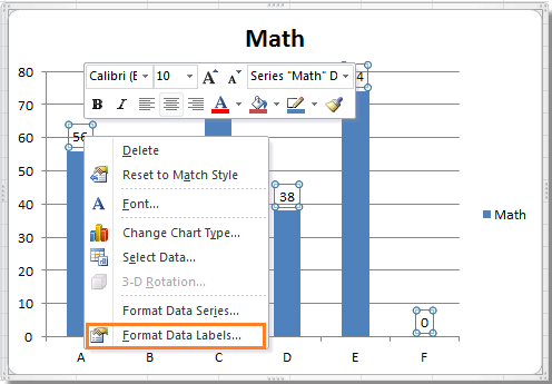
How to add data labels in excel to graph or chart (Step-by-Step) 1. Select a data series or a graph. After picking the series, click the data point you want to label. 2. Click Add Chart Element Chart Elements button > Data Labels in the upper right corner, close to the chart. 3. Click the arrow and select an option to modify the location. 4. How to Remove Zero Data Labels in Excel Graph (3 Easy Ways) Method-3: Using Custom Number Format to Format Data Labels of Chart. Without data labels, column charts may ignore zero data labels, but when we activate the data label option of the chart we can see the zero data labels for the Physics and Maths series also in the chart. To remove this label you can follow this section.

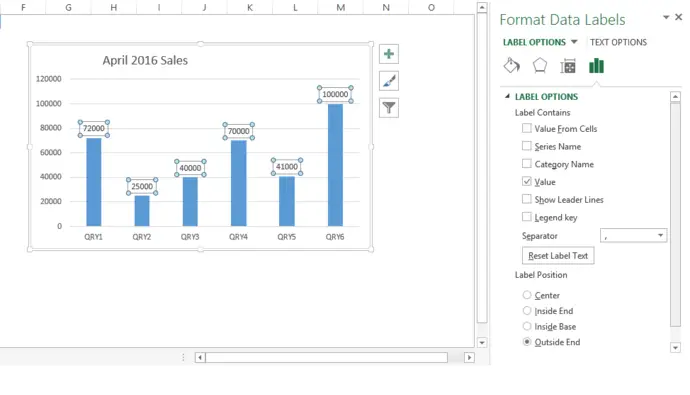
Using the CONCAT function to create custom data labels for ... Use the chart skittle (the "+" sign to the right of the chart) to select Data Labels and select More Options to display the Data Labels task pane. Check the Value From Cells checkbox and select the cells containing the custom labels, cells C5 to C16 in this example.

Excel chart custom data labels

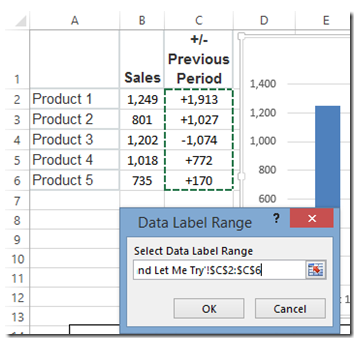
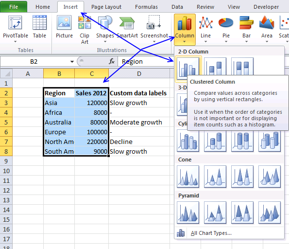
How to Use Cell Values for Excel Chart Labels Select the chart, choose the "Chart Elements" option, click the "Data Labels" arrow, and then "More Options." Uncheck the "Value" box and check the "Value From Cells" box. Select cells C2:C6 to use for the data label range and then click the "OK" button. The values from these cells are now used for the chart data labels. Xlsxwriter Excel Chart Custom Data Label Position At default the custom labels seem to bet set at right. I want them on top but I cant get this. The code is like that: chart.add_series ( .., 'data_labels': {'custom': my_custom_labels, 'position': 'above'}) But the changes wont appy to the chart. I also found i can set the default label position (label_position_default) in the chart object ... How to add data labels from different column in an Excel chart? Right click the data series in the chart, and select Add Data Labels > Add Data Labels from the context menu to add data labels. 2. Click any data label to select all data labels, and then click the specified data label to select it only in the chart. 3.

Excel chart custom data labels. Edit titles or data labels in a chart - support.microsoft.com The first click selects the data labels for the whole data series, and the second click selects the individual data label. Right-click the data label, and then click Format Data Label or Format Data Labels. Click Label Options if it's not selected, and then select the Reset Label Text check box. Top of Page Add / Move Data Labels in Charts - Excel & Google Sheets Add and Move Data Labels in Google Sheets Double Click Chart Select Customize under Chart Editor Select Series 4. Check Data Labels 5. Select which Position to move the data labels in comparison to the bars. Final Graph with Google Sheets After moving the dataset to the center, you can see the final graph has the data labels where we want. How to Customize Your Excel Pivot Chart Data Labels The Data Labels command on the Design tab's Add Chart Element menu in Excel allows you to label data markers with values from your pivot table. When you click the command button, Excel displays a menu with commands corresponding to locations for the data labels: None, Center, Left, Right, Above, and Below. Add Custom Labels to x-y Scatter plot in Excel Step 1: Select the Data, INSERT -> Recommended Charts -> Scatter chart (3 rd chart will be scatter chart) Let the plotted scatter chart be. Step 2: Click the + symbol and add data labels by clicking it as shown below. Step 3: Now we need to add the flavor names to the label. Now right click on the label and click format data labels.

How to create Custom Data Labels in Excel Charts Create the chart as usual Add default data labels Click on each unwanted label (using slow double click) and delete it Select each item where you want the custom label one at a time Press F2 to move focus to the Formula editing box Type the equal to sign Now click on the cell which contains the appropriate label Press ENTER That's it. Custom data labels in a chart - Get Digital Help Add data labels Press with right mouse button on on a column Press with left mouse button on "Add Data Labels" Double press with left mouse button on a data label Deselect Value Select Category name Press with left mouse button on Close Get the Excel file Custom-data-labels-in-a-chartv3.xlsx Charts category Add pictures to a chart axis Adding rich data labels to charts in Excel 2013 | Microsoft 365 Blog Putting a data label into a shape can add another type of visual emphasis. To add a data label in a shape, select the data point of interest, then right-click it to pull up the context menu. Click Add Data Label, then click Add Data Callout . The result is that your data label will appear in a graphical callout. Add or remove data labels in a chart - support.microsoft.com Click the data series or chart. To label one data point, after clicking the series, click that data point. In the upper right corner, next to the chart, click Add Chart Element > Data Labels. To change the location, click the arrow, and choose an option. If you want to show your data label inside a text bubble shape, click Data Callout.

Excel charts: add title, customize chart axis, legend and data labels Click the Chart Elements button, and select the Data Labels option. For example, this is how we can add labels to one of the data series in our Excel chart: For specific chart types, such as pie chart, you can also choose the labels location. For this, click the arrow next to Data Labels, and choose the option you want. Custom Data Labels with Colors and Symbols in Excel Charts - [How To] The basic idea behind custom label is to connect each data label to certain cell in the Excel worksheet and so whatever goes in that cell will appear on the chart as data label. So once a data label is connected to a cell, we apply custom number formatting on the cell and the results will show up on chart also. Apply Custom Data Labels to Charted Points - Peltier Tech There are a number of ways to apply custom data labels to your chart: Manually Type Desired Text for Each Label Manually Link Each Label to Cell with Desired Text Use the Chart Labeler Program Use Values from Cells (Excel 2013 and later) Write Your Own VBA Routines Manually Type Desired Text for Each Label Custom Chart Data Labels In Excel With Formulas Follow the steps below to create the custom data labels. Select the chart label you want to change. In the formula-bar hit = (equals), select the cell reference containing your chart label's data. In this case, the first label is in cell E2. Finally, repeat for all your chart laebls.

Formula Friday - Using Formulas To Add Custom Data Labels To Your Excel Chart - How To Excel At ...

How to add or move data labels in Excel chart? - ExtendOffice In Excel 2013 or 2016. 1. Click the chart to show the Chart Elements button . 2. Then click the Chart Elements, and check Data Labels, then you can click the arrow to choose an option about the data labels in the sub menu. See screenshot: In Excel 2010 or 2007. 1. click on the chart to show the Layout tab in the Chart Tools group. See ...

30 What Is A Data Label In Excel - Labels Database 2020

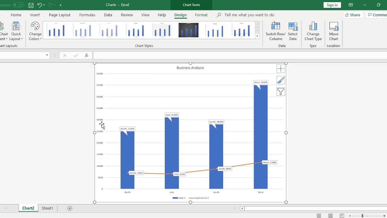
Add data labels and callouts to charts in Excel 365 | EasyTweaks.com Step #1: After generating the chart in Excel, right-click anywhere within the chart and select Add labels . Note that you can also select the very handy option of Adding data Callouts. Step #2: When you select the "Add Labels" option, all the different portions of the chart will automatically take on the corresponding values in the table ...

Excel Charts | How to Create a Chart in Excel | MS Excel in Hindi

Custom Excel Chart Label Positions - My Online Training Hub Custom Excel Chart Label Positions - Setup. The source data table has an extra column for the 'Label' which calculates the maximum of the Actual and Target: The formatting of the Label series is set to 'No fill' and 'No line' making it invisible in the chart, hence the name 'ghost series': The Label Series uses the 'Value ...

Custom Data Labels with Colors and Symbols in Excel Charts - [How To] - PakAccountants.com

Example: Charts with Data Labels - XlsxWriter Documentation Chart 1 in the following example is a chart with standard data labels: Chart 6 is a chart with custom data labels referenced from worksheet cells: Chart 7 is a chart with a mix of custom and default labels. The None items will get the default value. We also set a font for the custom items as an extra example: Chart 8 is a chart with some ...

Custom data labels in a chart | Get Digital Help - Microsoft Excel resource

Excel Custom Chart Labels • My Online Training Hub Custom Excel Chart Label Positions using a dummy or ghost series to force the label position neatly above the columns of data Lookup Pictures in Excel Lookup Pictures in Excel using values in cells returned by data validation lists (drop down lists) or Slicers. No VBA/Macros required!

Moving X-axis labels at the bottom of the chart below negative values in Excel - PakAccountants.com

How to add text labels on Excel scatter chart axis - Data Cornering Here is the data that I would like to display in the Excel scatter chart. In addition, I would like to add custom labels on Excel scatter chart x-axis with each person's name. Stepps to add text labels on Excel scatter chart axis. 1. Firstly it is not straightforward. Excel scatter chart does not group data by text.

How to Add Data Labels to your Excel Chart in Excel 2013 - YouTube

Improve your X Y Scatter Chart with custom data labels 2.3 How to use macro. Select the x y scatter chart. Press Alt+F8 to view a list of macros available. Select "AddDataLabels". Press with left mouse button on "Run" button. Select the custom data labels you want to assign to your chart. Make sure you select as many cells as there are data points in your chart.

Custom Data Labels with Colors and Symbols in Excel Charts - [How To] - PakAccountants.com

Excel Charts: Creating Custom Data Labels - YouTube Excel Charts: Creating Custom Data Labels 84,148 views Jun 26, 2016 191 Dislike Share Save Mike Thomas 4.48K subscribers Subscribe In this video I'll show you how to add data labels to a chart in...

excel - How do I update the data label of a chart? - Stack Overflow

How to Change Excel Chart Data Labels to Custom Values? You can change data labels and point them to different cells using this little trick. First add data labels to the chart (Layout Ribbon > Data Labels) Define the new data label values in a bunch of cells, like this: Now, click on any data label. This will select "all" data labels. Now click once again.

10 Design Tips to Create Beautiful Excel Charts and Graphs in 2017

» Excel Charts: Creating Custom Data Labels In this video I'll show you how to add data labels to a chart and then change the range that the data labels are linked to. If you are using Excel 2013 or above on Windows, there is a simple way to do this. However if you're using an earlier version or you're using Excel 2106 on the Mac, it's more of a manual process. The video covers both.

How to hide zero data labels in chart in Excel?

How to add data labels from different column in an Excel chart? Right click the data series in the chart, and select Add Data Labels > Add Data Labels from the context menu to add data labels. 2. Click any data label to select all data labels, and then click the specified data label to select it only in the chart. 3.

Creating a chart with dynamic labels - Microsoft Excel 2016

Xlsxwriter Excel Chart Custom Data Label Position At default the custom labels seem to bet set at right. I want them on top but I cant get this. The code is like that: chart.add_series ( .., 'data_labels': {'custom': my_custom_labels, 'position': 'above'}) But the changes wont appy to the chart. I also found i can set the default label position (label_position_default) in the chart object ...