40 conditional formatting pivot table row labels

Pivot Table Conditional Formatting with VBA - Peltier Tech A reader encountered problems applying conditional formatting to a pivot table. I tried it myself, using the same kind of formulas I would have applied in a regular worksheet range, and had no problem. ... including what I think you meant with your last suggestions (and Text1 is one of my Row Labels, and Text is one of the names populating ... Excel VBA: Conditional Format of Pivot Table based on Column Label myPivotSourceName = myPivotField.Name. Then rather than referencing the data field with the pivot field object, I referenced the DataRange with the string: myPivotTable.PivotFields (myPivotSourceName).DataRange.Select. Works perfectly and is completely portable for any pivottable on any sheet with any fields. excel vba.

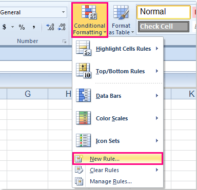
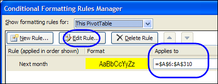
Add Pivot Table Conditional Formatting and Fix Problems This step will prevent conditional formatting problems after you refresh the pivot table. Select any cell in the pivot table On the Ribbon's Home tab, click Conditional Formatting, then click Manage Rules The Conditional Formatting Rules Manager opens, where you can create a new rule, edit an existing rule, or delete a rule

Conditional formatting pivot table row labels

Pivot Table Conditional Formatting Based on Another Column (8 Easy Ways ... We'll use a single selected cell to apply conditional formatting to the entire Quantity column of the Pivot Table. Step 1: Select any single cell (i.e., C4 ). Then Go to Home Tab > Select Conditional Formatting (in Styles section) > Choose New Rule. Step 2: New Formatting Rule window opens up. In the window, select the 3rd option in the Apply ... Pivot Table Grouping, Ungrouping And Conditional Formatting So let's drag the Age under the Rows area to create our Pivot table. #1) Right-click on any number in the pivot table. #2) On the context menu, click Group. #3) Grouping dialog box appears, in this example, the least number is 25, so by default the Starting number is entered as 25, and you can change if necessary. How to Apply Conditional Formatting to Rows Based on Cell Value On the Home tab of the Ribbon, select the Conditional Formatting drop-down and click on Manage Rules…. That will bring up the Conditional Formatting Rules Manager window. Click on New Rule. This will open the New Formatting Rule window. Under Select a Rule Type, choose Use a formula to determine which cells to format.

Conditional formatting pivot table row labels. Conditional formatting rows in a pivot table based on one rows criteria ... I am havong difficulty trying to highlight an entire row in a pivot table based on one rows criteria. The pivot table is from A:M and I need to highlight the corresponding row if column I has 992 in it. I have tried sevral ways but can only get it to work if I just focus on one row. I am at a loss for what I am doing wrong. How to Apply Conditional Formatting to Pivot Tables So in this post I explain how to apply conditional formatting for pivot tables. 1. Select a cell in the Values area The first step is to select a cell in the Values area of the pivot table. If your pivot table has multiple fields in the Values area, select a cell for the field you want to apply the formatting to. 2. Apply Conditional Formatting Pivot Table Conditional Formatting Weekend Data Highlight There are 3 main steps in setting up this pivot table conditional formatting, and the details for each step are shown in the sections below: -- 1) Create Formula for Weekend Dates -- 2) Add Conditional Formatting Rule to Pivot Table -- 3) Adjust Conditional Formatting Rule 1) Create Formula for Weekend Dates Pivot Table Conditional Formatting for Different Rows Items? Hello, It is possible! All you have to do: Select Your Pivot Table and: Go to Conditional Formatting -> New Rule -> Choose All cells showing "duration" values for "Type and "Date Selection" under "Apply Rule To" section -> Use a Formula to Determine which cells to format and enter the following formula: =AND(A6="Cars",A6>3), You can create new rules for other two conditions as well:

Using column label as formatting condition in excel pivot table I have pivot table in excel with sample data as attached. I now want to apply conditional formatting as red background where - data is between 10 to 25 AND - year is 2011 and 2012. =AND(C1="2011",OR(C2>10,C2<25)) how do i make cells example c2,c3,d2 red based on condition of year. Without Year condition it is working fine. Conditional Formatting in Pivot Table (Example) | How To Apply? Click on any cell in the pivot table > Go to the HOME tab > Click on Conditional Formatting option under Styles option > Click on Manage Rules option. It will open a Rules Manager dialog box. Click on the Edit Rule tab, as shown in the below screenshot. It will open the Editing Rule formatting window. Refer to the below screenshot. How to conditional formatting pivot table in Excel? Conditional formatting pivot table. 1. Select the data range you want to conditional formatting, then click Home > Conditional Formatting.. Note: You only can conditional formatting the Field in Values section in the PivotTable Field List Pane.. 2. Then in the popped out list, select the conditional formatting rule you need, here I select Data Bars for instance. Conditional Formatting PivotTables - My Online Training Hub Here's a step by step how to: 1. Select any cell in the values area of your PivotTable. 2. On the Home tab of the Ribbon select Conditional Formatting > Top/Bottom Rules > Top 10 Items: 3. Set the value to 1 and choose your format: 4. You will now have an icon beside the cell that you have applied the formatting to.

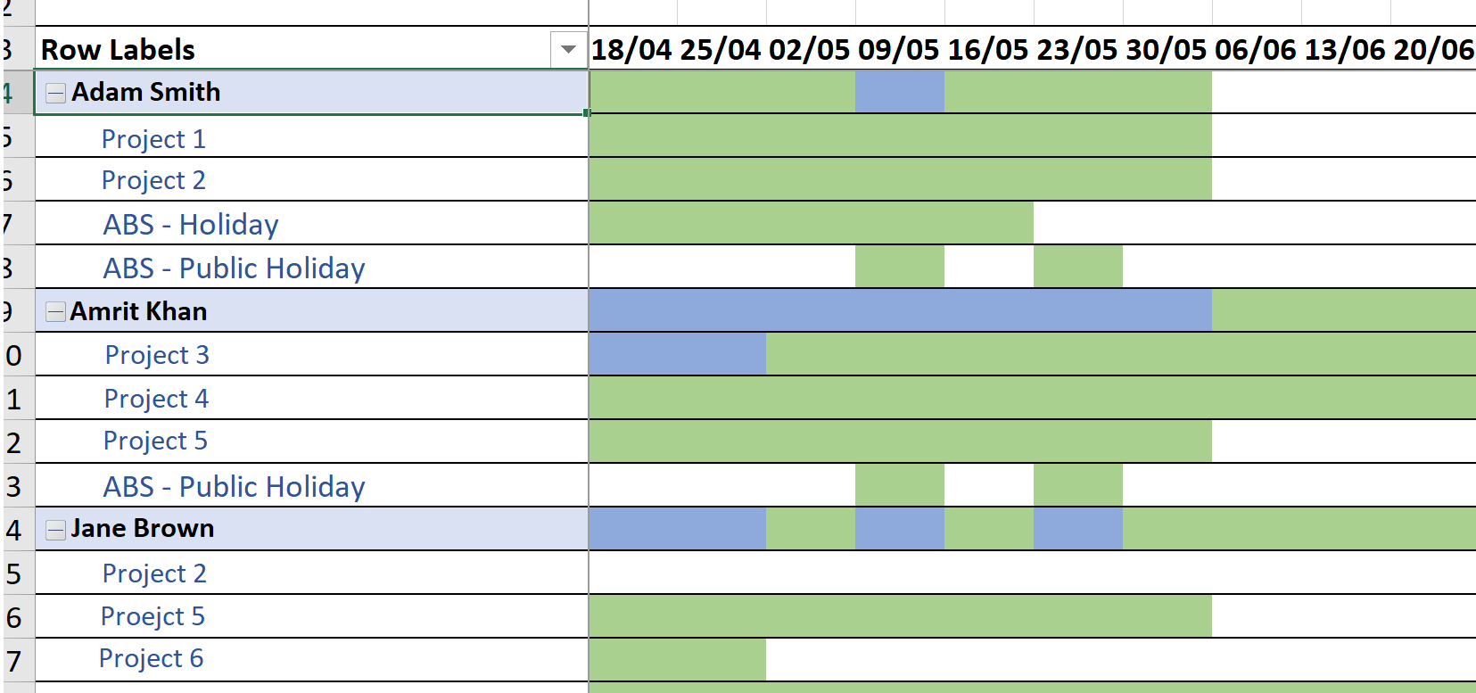
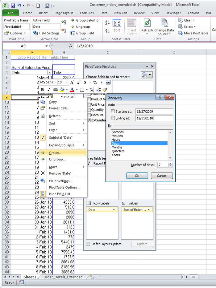
Format Pivot Table Labels Based on Date Range In the pivot table, remove any filters that have been applied - all the rows need to be visible before you apply the conditional formatting. Select all the dates in the Row Labels that you want to format. On the Ribbon, click the Home tab, and then in the Styles group, click Conditional Formatting. Conditional Format Pivot Table Row - Chandoo.org Select the entire row, and when you apply the conditional format, make the column reference absolute. So, say we want the entire row 2 to be formatted if cell in col B = 5. formula would be: =$B2=5 Re-Apply Pivot Table Conditional Formatting - yoursumbuddy So, I wrote the code below to expand the condtional formatting from the first row label cell into all the row label and data area cells: Sub Extend_Pivot_CF_To_Data_Area () Dim pvtTable As Excel.PivotTable Dim rngTarget As Excel.Range Dim rngSource As Excel.Range Dim i As Long 'check for inapplicable situations If ActiveSheet Is Nothing Then Conditional Formatting on Pivot Table row labels In srcFromPowerPivot sheet cell A is from powerpivot under row label comparing the dates in cell C (3 dates) and the condtional formatting doesnt work. In cell J it worked cos I dragged under value instead of row label. In the srcFromWorksheet it worked even though it is under rowlabel. Sheet3 is just a copy of powerpivot data.

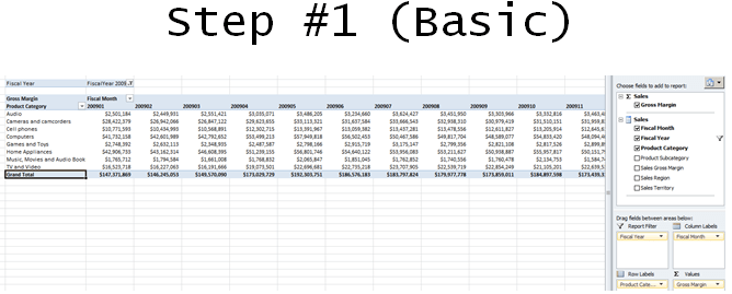
How to train your users to create their own Business Intelligence reports? #4 of 5: Sample ...

Overwrite pivot table conditional format based on row label As far as I know, using the one rule in the Conditional formatting, we can only format the cells with one color if the condition is true and if the same condition is false, the formatting of the cell will be blank and if both conditions are true, the formatting of cell depends on the highest ranking/priority of the rules in Conditional formatting.

Insert Grand Totals to a Pivot Table - Free Microsoft Excel Tutorials

Pivot table conditional formatting - Exceljet The best option is to set up the the rule correctly from the start. Select any cell in the data you wish to format and then choose "New rule" from the conditional formatting menu on the Home tab of the ribbon. At the top of the window, you will see setting for which cells to apply conditional formatting to. For the example shown, we want:

How to Apply Data Bars in Pivot Table - MS Excel | Excel In Excel

Pivot table conditional formatting based on row label jobs Search for jobs related to Pivot table conditional formatting based on row label or hire on the world's largest freelancing marketplace with 21m+ jobs. It's free to sign up and bid on jobs.

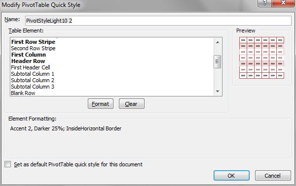
Unified Method of Pivot Table Formatting - yoursumbuddy

Apply Conditional Formatting | Excel Pivot Table Tutorial Go to Home Tab → Styles → Conditional Formatting → New Rule. From rule to, select the third option. And, from "select a rule" type select "Format only top or bottom" ranked values. In edit rule description, enter 1 in the input box and from the drop-down menu select "each Column Group". Apply formatting you want. Click OK.

How to remove bold font of pivot table in Excel?

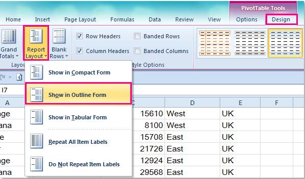
Design the layout and format of a PivotTable Right-click the field name and then select the appropriate command — Add to Report Filter, Add to Column Label, Add to Row Label, or Add to Values — to place the field in a specific area of the layout section. Click and hold a field name, and then drag the field between the field section and an area in the layout section.

Learn How to Apply Conditional Formatting in a Pivot Table | Excelchat

Conditional formatting for Pivot Tables in Excel 2016 - Ablebits Conditional formatting when applied to PivotTables in Excel 2007 - 2016 is applied to the underlying structure of the PivotTable rather than to the cells themselves. So, when you interact with a PivotTable such as moving fields around and viewing your data in different ways, the formatting is updated as you work.

How to Create a MS Excel Pivot Table – An Introduction | SIMPLE TAX INDIA

Conditional Formatting in Pivot Table - WallStreetMojo We must follow the steps to apply conditional formatting in the pivot table. First, we must select the data. Then, in the "Insert" Tab, click on "Pivot Tables." As a result, a dialog box appears. Next, we must insert the pivot table in a new worksheet by clicking "OK." Currently, a pivot table is blank. Next, we need to bring in the values.

How to repeat row labels for group in pivot table?

Excel Pivot Table Conditional Formatting Row Labels Go making the conditional formatting select the color scale and do it based on commercial and choose diverging and the colors should give expected result. Here a glaze color or bar and been applied...

Format Pivot Table Labels Based on Date Range – Excel Pivot Tables

How to make row labels on same line in pivot table? Make row labels on same line with PivotTable Options You can also go to the PivotTable Options dialog box to set an option to finish this operation. 1. Click any one cell in the pivot table, and right click to choose PivotTable Options, see screenshot: 2.

Insert Subtotals to a Pivot Table - Free Microsoft Excel Tutorials

How to Apply Conditional Formatting to Rows Based on Cell Value On the Home tab of the Ribbon, select the Conditional Formatting drop-down and click on Manage Rules…. That will bring up the Conditional Formatting Rules Manager window. Click on New Rule. This will open the New Formatting Rule window. Under Select a Rule Type, choose Use a formula to determine which cells to format.

Conditional formatting in Pivot Tables - Goodly

Pivot Table Grouping, Ungrouping And Conditional Formatting So let's drag the Age under the Rows area to create our Pivot table. #1) Right-click on any number in the pivot table. #2) On the context menu, click Group. #3) Grouping dialog box appears, in this example, the least number is 25, so by default the Starting number is entered as 25, and you can change if necessary.

Conditional Formatting in Pivot Table (Example) | How To Apply?

Pivot Table Conditional Formatting Based on Another Column (8 Easy Ways ... We'll use a single selected cell to apply conditional formatting to the entire Quantity column of the Pivot Table. Step 1: Select any single cell (i.e., C4 ). Then Go to Home Tab > Select Conditional Formatting (in Styles section) > Choose New Rule. Step 2: New Formatting Rule window opens up. In the window, select the 3rd option in the Apply ...

Overwrite pivot table conditional format based on row label - Microsoft Community

How To Group Data In Excel Based On A Column Value - get a list of distinct unique values in ...

How to Sort Pivot Table Row Labels, Column Field Labels and Data Values with Excel VBA Macro ...

How to use conditional formatting in decorating pivot tables | Basic Excel Tutorial

Conditional formatting based on the values in another table | Page 2 | Access World Forums

vba - Conditional Formatting in Pivot Table in Excel based on text field - Stack Overflow

Share :